This content is for members only.
Already have an account? Login
In this article, we will talk about
- Limitations of Deep Neural Networks
- Motivation for Recurrent Neural Networks
- Example of a Sequence Problem - Named Entity Recognition
- RNN Architecture
- Training a Recurrent Network
This article assumes you are familiar with Vanilla Neural Networks (also known as Multi-Layer Perceptrons) and the basic concepts of Linear Algebra that are used in Deep Learning. Knowledge about a few activation functions (like ReLU and Sigmoid) and loss functions (like Binary Cross Entropy Loss) that are used in standard classification models is a prerequisite.
$$
\begin{array}{cccc}
\begin{bmatrix}0 \\ 0 \end{bmatrix} \rightarrow \begin{bmatrix}0 \end{bmatrix} &
\begin{bmatrix}0 \\ 1 \end{bmatrix} \rightarrow \begin{bmatrix}0 \end{bmatrix} &
\begin{bmatrix}1 \\ 0 \end{bmatrix} \rightarrow \begin{bmatrix}0 \end{bmatrix} &
\begin{bmatrix}1 \\ 1 \end{bmatrix} \rightarrow \begin{bmatrix}1 \end{bmatrix}
\end{array}
$$
It is a significant limitation, since many important problems are best expressed with sequences whose lengths are not known beforehand. A simple example of a sequence problem is question answering which can be seen as mapping a sequence of words representing the question to a sequence of words representing the answer.
$$
\begin{array}{cc}
\begin{bmatrix} \text{How} \\ \text{was} \\ \text{your} \\ \text{day?} \end{bmatrix} \rightarrow \begin{bmatrix} \text{It} \\ \text{was} \\ \text{good} \end{bmatrix}
& \quad \quad
\begin{bmatrix} \text{Did} \\ \text{Ram} \\ \text{eat} \\ \text{rice} \\ \text{today?} \end{bmatrix} \rightarrow \begin{bmatrix} \text{Yes} \end{bmatrix}
\end{array}
$$
In such problems, the lengths of input and output sequence are not known beforehand. For different input sequences, the length of different output sequences can be different. It is therefore clear that a network that learns to map sequences to sequences would be useful. This is where Recurrent Neural Networks (RNNs) can be helpful. To explain how RNN works, let's take a similar but simpler example of Named Entity Recognition.
Named Entity Recognition
Suppose the problem given is to identify names of people in a sentence. We can represent this problem as follows. If the sentence is given as words in an array, we can assign a $1$ or $0$ to each word which signifies if the word is part of a name or not. In this case, out input and output to the network would look like so
$$\begin{array}{l} \text{input : } \quad \ \ \text{Harry Potter and Hermione Granger invented a new spell} \\ \text{output : } \quad [1, 1, 0, 1, 1, 0, 0, 0, 0] \end{array}$$
We will use the following notations to represent individual words in a input sentence and the values of output sequence
$$\begin{array}{l} \text{input :} \quad \ \ \ \ \ \ \text{Harry Potter and Hermione Granger invented a new spell} \\ \text{Notation :} \quad [x^{<1>}, x^{<2>}, x^{<3>}, \dots \quad \dots x^{<t>} \dots \quad \dots x^{<9>}] \\ \\ \text{output :} \quad \ \ \ \ [1, 1, 0, 1, 1, 0, 0, 0, 0] \\ \text{Notation :} \quad [y^{<1>}, y^{<2>}, y^{<3>}, \dots \quad \dots y^{<t>} \dots \quad \dots y^{<9>}] \end{array}$$
Some other notations that we will use in our analysis are
$$\begin{array}{l} T_x = 9 \quad \text{(Length of input sequence)} \\ T_y = 9 \quad \text{(Length of output sequence)} \end{array}$$
In this example, $T_x$ and $T_y$ are same but for different problems they can be of different lengths. How do we handle this? This is where the "recurrent" part of recurrent neural network helps us.
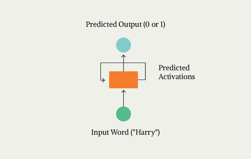
The main idea of RNN is to have a single independent processing unit (which processes a single word) and re-use this same unit for all the words in the sentence. Think of it like a magic box. You give the box a word as input (say Harry) and it outputs 0 or 1 depending on whether the word is part of a name or not. For other words in the sentence, you re-use this same box by providing it the next word ("Potter") and having it do exactly the same thing again.
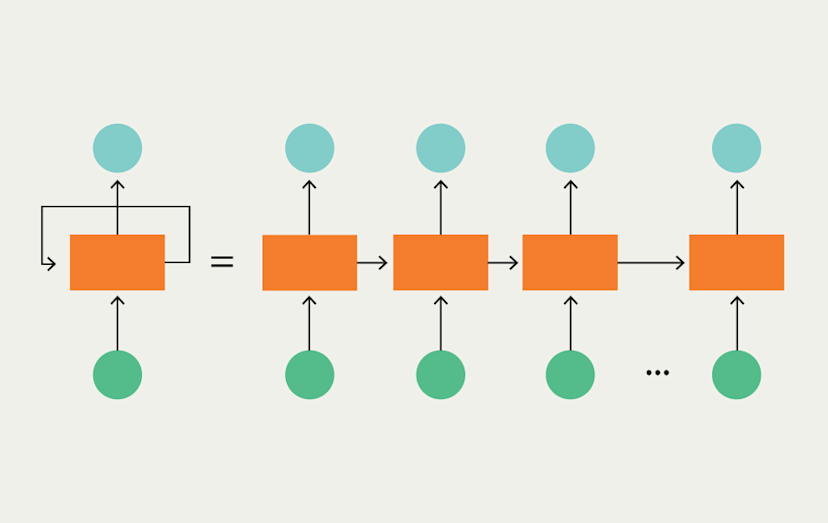
Since this is a sequential process (process first word, then second, then third), we can allow the box to have more context about each word by predicting a set of "activations" along with our 0/1 output. We can then pass the activations as input along with the next word. This is why RNNs are sometimes depicted like so:
This diagram is sometimes also called "rolled" RNN. Since, each time we use the same recurrent unit to process a new word in the sentence, we refer to this single processing task as a timestep. In each timestep, we process a single word and over multiple timesteps we process the entire sentence.
Since our training dataset will have multiple training examples (input and output), we have
$$\begin{array}{l} T_x^{(i)} : \quad \text{Length of } i^{th} \text{ training example (input sequence length)} \\ T_y^{(i)} : \quad \text{Length of } i^{th} \text{ training example (output sequence length)} \\ \\ X^{(i)\langle t \rangle} : \quad t^{th} \text{ element (word) in } i^{th} \text{ training example (input)} \\ Y^{(i)\langle t \rangle} : \quad t^{th} \text{ element (value) in } i^{th} \text{ training example (output)} \end{array}$$
Recurrent Neural Network Architecture
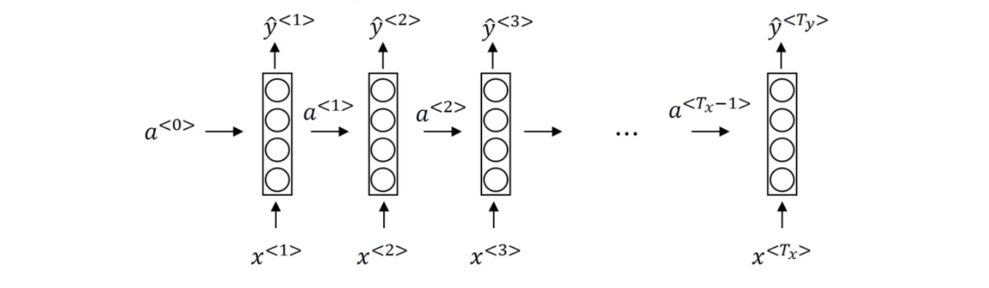
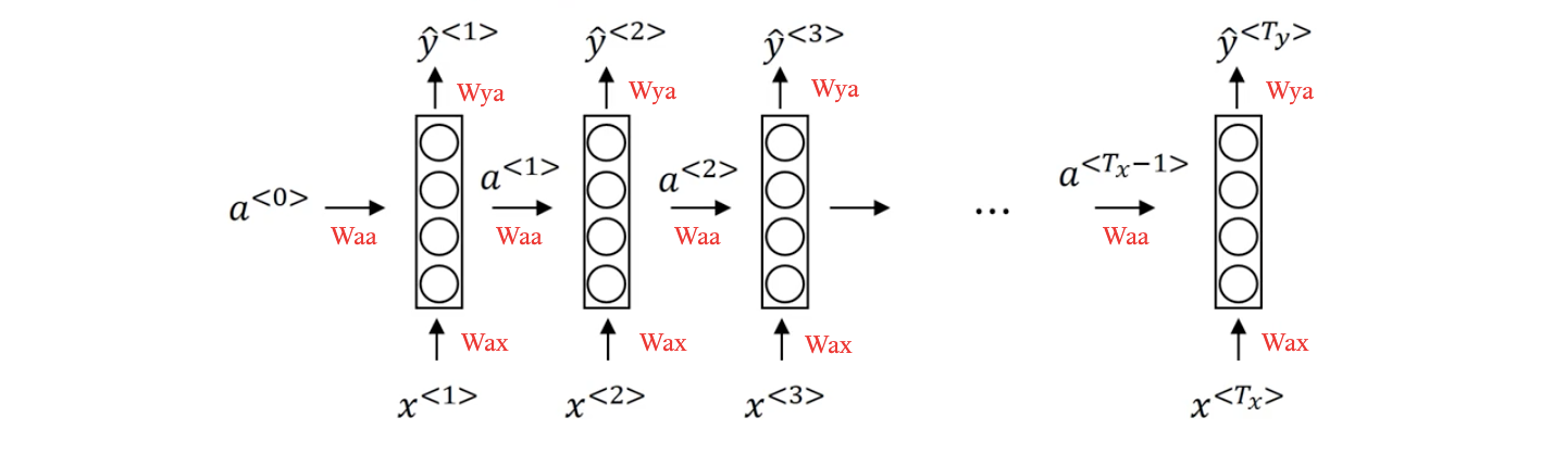
Each $x^{<t>}$ is given to a input layer, along with a vector of activations $a^{<t-1>}$ to compute an output prediction $\hat{y}^{<t>}$ and the vector of activations for next timestep After processing $x^{<t>}$, when we process the next word $x^{<t+1>}$, we use the activations generated from the previous layer $a^{<t>}$ along with next input to predict the next output $\hat{y}^{<t+1>}$ and next activations. This process continues until the entire input sequence gets processed. We use 3 sets of parameters $W_{ax}$, $W_{aa}$, and $W_{ya}$ which will govern the connections from current input $x^{<t>}$, connection from previous activations $a^{<t-1>}$, and connection to output $\hat{y}^{<t>}$. All of these sets of parameters are used again and again (recurrently) for every word as shown in the diagram below
To compute the predictions $\hat{y}^{<t>}$ and activations $a^{<t>}$ in first layer, we will use the following equations:
- $a^{<0>} = \vec{0}$ (By Default)
- $a^{<1>} = g_1(W_{aa}\ a^{<0>} + W_{ax}\ x^{<1>} + b_a)$
- $\hat{y}^{<1>} = g_2(W_{ya}\ a^{<1>} + b_y)$
$g_1(x)$ can be $tanh(x)$ or ReLU and $g_2(x)$ can be sigmoid or softmax activation function. A quick tip to remember which set of weights should be multiplied with what is to remember the following:
- $W_{ax}$ : The second subscript $x$ means that these weights are to be multiplied with some $x$ like quantity and the first subscript $a$ means that these weights are used to predict some $a$ like quantity.
- $W_{ya}$ : Similarly, this should be multiplied with some $a$ like quantity to predict some $y$ like quantity.
We can also generalize these equation for any timestep as follows:
- $a^{<0>} = \vec{0}$
- $a^{<t>} = g_1(W_{aa}\ a^{<t-1>} + W_{ax}\ x^{<t>} + b_a)$
- $\hat{y}^{<t>} = g_2(W_{ya}\ a^{<t>} + b_y)$
Training a Recurrent Neural Network
Since RNNs compute a predicted output $\hat{y}^{<t>}$ for each timestep $t$ and we expect a correct output $y^{<t>}$ for each word, we can use a loss function to calculate how good or bad the prediction was and use it to train the network. Since it is a sequential process, a loss (or error) will be computed for each timestep first and since this problem is similar to a classification problem (classify each word as 0 or we can use a Binary Cross Entropy Loss (BCE) for each $\hat{y}^{<t>}$.
$$\mathcal{L}^{\langle t \rangle}(\hat{y}^{\langle t \rangle}, y^{\langle t \rangle}) = -\hat{y}^{\langle t \rangle} \log(\hat{y}^{\langle t \rangle}) - (1 - y^{\langle t \rangle}) \log(1 - \hat{y}^{\langle t \rangle})$$
The overall loss for the entire network can then be computed as follows:
$$\mathcal{L} = \sum_{t=1}^{T_{y}} \mathcal{L}^{\langle t \rangle}(\hat{y}^{\langle t \rangle}, y^{\langle t \rangle})$$
Since the loss is one layer (one time step) depends upon the activations from the previous layer (previous time step), a dependency chain is formed. To train the network, we need to update the gradients from the last later (last timestep) and then go backwards to the first layer (first timestep). This is sometimes called "Back Propagation Through Time".
To adjust the weights using gradients, an optimizer like Adaptive Moment Estimation (ADAM) or RMSprop can be used. Since these are widely used in other deep learning areas and not just RNN, we skip their descriptions here and will cover them in a different post.
That's it for this post! In this article, we covered what RNNs are, how they work, their architecture and the internal mathematics. We also saw how RNNs can be applied to a Sequence Learning problem (Named Entity Recognition). In reality, many different NLP problems like translation, text generation, and sentiment analysis can be solved using RNNs. We will also try to cover some of them in the upcoming posts. Till then, if you have any questions or suggestions on this topic, please do let us know in the comment and we'll be happy to help you out. Stay safe and Happy Learning!